

23.03.2024

ENHANCING SPACE SITUATIONAL AWARENESS TO MITIGATE RISK: A CASE STUDY IN THE MISIDENTIFICATION OF STARLINK SATELLITES AS UAP IN COMMERCIAL AVIATION
Douglas J. Buettner(1)(2)(3)*, Richard E. Griffiths(4)(5), Nick Snell(1), and John Stilley(1)
(1)Department of Mechanical Engineering, University of Utah,
1495 E 100 S (1550 MEK), Salt Lake City, UT 84112, 801.581.6441, doug.buettner@utah.edu
(2)Acquisition Innovation Research Center, Stevens Institute of Technology, 1 Castle Point Terrace, Hoboken, NJ 07030, USA, 201.216.8300, airc@acqirc.org
(3)Sr. Member of the AIAA
(4)Department of Physics & Astronomy, University of Hawaii at Hilo, 200 W. Kawili St., Hilo, HI 96720, USA, 808.339.4760, griff2@hawaii.edu (5)Department of Physics, Carnegie Mellon University, 5000 Forbes Ave., Pittsburgh, PA 15213, USA, 808.339.4760, rgriff@andrew.cmu.edu
∗To whom correspondence should be addressed
Keywords: satellite constellations, Starlink, simulation, rendering, specular reflection,
aviation risk, UAP, astrometry
ABSTRACT
Over the past several years, the misidentification of SpaceX/Starlink satellites as Unidentified Aerospace Phenomena (UAP) by pilots and laypersons has generated unnecessary aviation risk and confusion. The many deployment and orbital evolution strategies, coupled with ever changing sun specular reflection angles, contribute to this gap in space situational awareness. While SpaceX/Starlink and other satellite operators are working on partial mitigations of this novel light pollution for the astronomical community, it is unlikely that these mitigations will resolve the misidentification of Starlinks as UAP for aviators and the public. In this paper we present a case analysis of an incident that generated multiple, corroborating reports of “a UAP” from five pilots on two commercial airline flights over the Pacific Ocean on August 10th, 20221. This incident included two cell phone photos and a video of an unrecognizable and possibly anomalous phenomenon. We then use supplemental two-line elements (TLEs) for the Starlink ’train’ of satellites launched that same day and Automatic Dependent Surveillance-Broadcast (ADS-B) data from the flight with the photographs to reconstruct a view of these satellites from the cockpit at the time and place of the sighting. The success of this work demonstrates an approach that could, in principle, warn aviators about satellites that could be visible in unusual or novel illumination configurations, thus increasing space situational awareness and supporting aviation safety. The approach is based on standard orbital mechanics and ray-traced rendering of the view from the pilots’ cockpit in visualization simulations. In the implementation of our approach, we were able to closely match the apparent speed in degrees per second traveled by the object between the two photographs taken by one of the pilots. Further, our rendering experiments suggest that the Starlink
1 One of the flights had a pilot who was in training, hence the total pilots observing the object were the captain, the co-pilot and the pilot in training satellite train would not have been visible if the solar arrays were not deployed. We then discuss the potential for this visualization approach to reduce unknown sightings that lead to pilot distraction and subsequent airwave chatter, through future work to fully simulate the range of deployment configurations with the sun’s relative location effect on the illumination of and specular reflections from these objects. We conclude with recommendations for government and satellite operators to provide better a-priori data that can be used to create advisories to aviators and the public. The automated simulation of known specular reflection off constellations of satellites could also support researchers investigating sightings of unfamiliar aerial/aerospace objects as likely being from normal versus novel space events.
1. Introduction
SpaceX/Starlink satellites misidentified as Unidentified Aerospace Phenomena (UAP) has generated significant press over the past few years (CBS Pittsburgh 2021, WCVB Channel 5 Boston 2023, Reyes 2023, Tangermann 2019, Grassi 2023, Mandelbaum 2019). While SpaceX is working to at least partially resolve this novel light pollution issue for the astronomical community (Tangermann 2019, Loeffler 2023, SpaceX 2022), we do not believe it will resolve the misidentification as UAP issue as recent videos of new Starlink 2.0 minis are still clearly visible (Schrader 2023, LIVE 2023).
In addition, recent US government congressional hearings about UAP and concomitant media attention about the alleged recovery of craft of extraterrestrial origin (117th Congress (2021-2022) 2022, C-SPAN 2023) has intrigued the public. The U.S. military, under congressional order, has set up a special office for collecting and addressing UAP reports from all current or former government employees, service members, or contractors (AARO 2024). In early 2024, a congressional bill related to flight safety was introduced that will help facilitate reporting of UAP sightings to the Federal Aviation Administration (FAA) by all commercial aviation personnel (Garcia 2024). As a result of these activities, people from many sectors are becoming acutely aware of what they are seeing in the sky, such that if they do not know what it is, they are now providing cell phone photographic and/or video evidence of their sighting. This increased awareness of an unresolved evidence trail of UAP sightings, and the consequent risks to aviation safety and national security, has resulted in a concerted effort to look beyond the dismissal of sightings as simply social and psychological phenomena (Sharps 2023, Torre 2024, Yingling 2023a, Yingling 2023b).
This is leading to a reduction of the stigma associated with the serious study of phenomena underlying 'Unidentified Flying Objects (UFO)' (Sultan 2023, Dunn 2023, Gallaudet and Mellon 2023, Williamson 2023). The once reluctant scientific community is slowly starting to consider the underlying causes of UAP reports as an interesting area for research (Yingling 2023a, Yingling 2023b, David 2023, Medina 2023, Watters, et al. 2023), with global reach (Lomas 2023). However, we lack sufficiently mature tools and methods to systematically analyze sighting reports for the "known phenomena" category. Without such critical methodologies in place, satellites, rockets, and drones will continue to clutter pilot communication channels and aviation hazard databases as these knowable lights in the sky are reported as UAP.
We start this paper with a case study describing a first attempt to analyze a corroborated UAP sighting over the Pacific Ocean from airline pilots, generally considered to be "trained observers" (Graves 2023, Schwartz 2022), one of whom also provided photographic evidence of the long, slender, and solid white object. At the time of reporting, the pilots were unaware of what a SpaceX/Starlink deployment could look like based on the analysis in this paper, in fact, news reports and online YouTube videos of the "string of pearls" Starlink satellites dominate the common perception of what one should see. Here we provide the raw observations which were reported to the worldwide Mutual UFO Network (MUFON) and recorded as MUFON case number 124190 and the subsequent analysis by one of us to characterize this UAP case using the available evidence at that time. We include this attempt here as a case study of extracting information on objects from photographic and astrometric evidence alone to advance the scientific study of UAP.
Following the case study, we describe an approach that researchers can use to filter out low-altitude satellites such as Starlinks, thus moving them from the "unknown" to the "known" category of witnessed events. The method uses tools from orbital mechanics and visualization simulation techniques. This method is in its infancy as we need to make assumptions about the deployment status (e.g. spacing, spacecraft attitude, and deployment of solar arrays) of these satellites. We conclude with recommendations regarding additional data required to support building an analytic capability that could provide notices in advance to aviators and the public about space- related events. We also identify future research to support a priori notifications and after-the-fact analysis of UAP sightings and reports.
2. TheObservationalCaseStudy Observations
Here we document the observations that were made from two separate aircraft flying on the same flight path over the Pacific Ocean in August of 2022. The lead aircraft was flight number AC536 flying from Maui to Vancouver B.C. The trailing aircraft was flight number AC34 flying from Sydney Australia to Vancouver B.C.
Four or five very bright unresolved star-like objects were seen by the captain and co- pilot of AC34, as reported by the airline captain (Pittet 2023). The individual objects brightened to be brighter than the International Space Station for a short period of time and then faded. The captain provided an estimated distance of 35-75 nautical miles when first sighted on his assumption that they were within the atmosphere at an altitude which was roughly the same as the airliner (a barometric altitude of ~39,000 ft). The captain watched these individual star-like objects fade and appear to converge into a single large, craft-like object.
This craft-like object then appeared to fly ahead and roughly parallel with the aircraft's flight path, at which point it came into the field of view of the leading aircraft AC534, on the same flight path. From this lead aircraft, the large craft could be observed moving parallel and just above the horizon, apparently at 37,000 ft., traversing an azimuthal angle of 90 degrees (from North-West to North-East) in about two minutes.
During the latter part of this flight, the apparent large craft ('cigar shaped' in projection) was photographed and videoed by an anonymous pilot of the lead plane (flight AC536) and confirmed visually by two other pilots on this same flight. The initial bright objects were not seen by the pilots of this latter flight because the objects were directly behind them, and the two aircraft were separated by about 160 miles.
The integrated brightness of the elongated object in the photos/video from the lead plane was very much less than the integrated brightness of the 4 to 5 objects originally observed by the trailing plane.
In all, observations of the large object were confirmed by five pilots with two cellphone photos (Figure 1 shows photo 1 taken at 2022-08-10T11:39:08UTC and Figure 2 shows photo 2 taken at 2022-08-10T11:39:24UTC) and a ~16-second video taken by the pilot on the leading plane. The video was bracketed by the two photos. The initial, separate, star-like objects were seen by the two pilots of the trailing plane only. The approximate longitude/latitude of the aircraft at the time of sighting was 39 degrees North, -133 degrees West, as determined from ’FlightRadar24’2. There were no radar records of any of the objects that were seen visibly by the pilots – the airliners (a Boeing 789 and a Boeing 38M) had onboard radar tuned for weather (forward-looking), but not for objects at large azimuthal angles relative to their heading vectors.
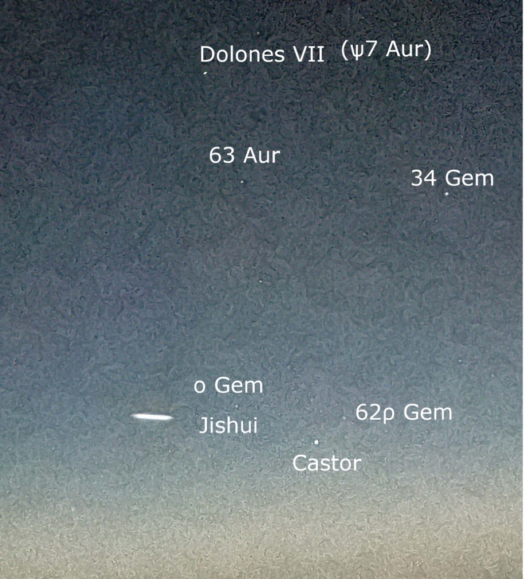
Figure 1. Photo 1 from an iPhone 12 camera taken at 2022-08-10T11:39:08UTC as determined by information embedded in the JPEG metadata. The astrometric solution to the starfield, i.e. the identification of the stars, was found using the publicly-available software package Astrometry.net. The object was observed at ~2 am local solar time when the aircraft was at a latitude of 39.60321 degrees North, and a longitude of 138.436 degrees West.3
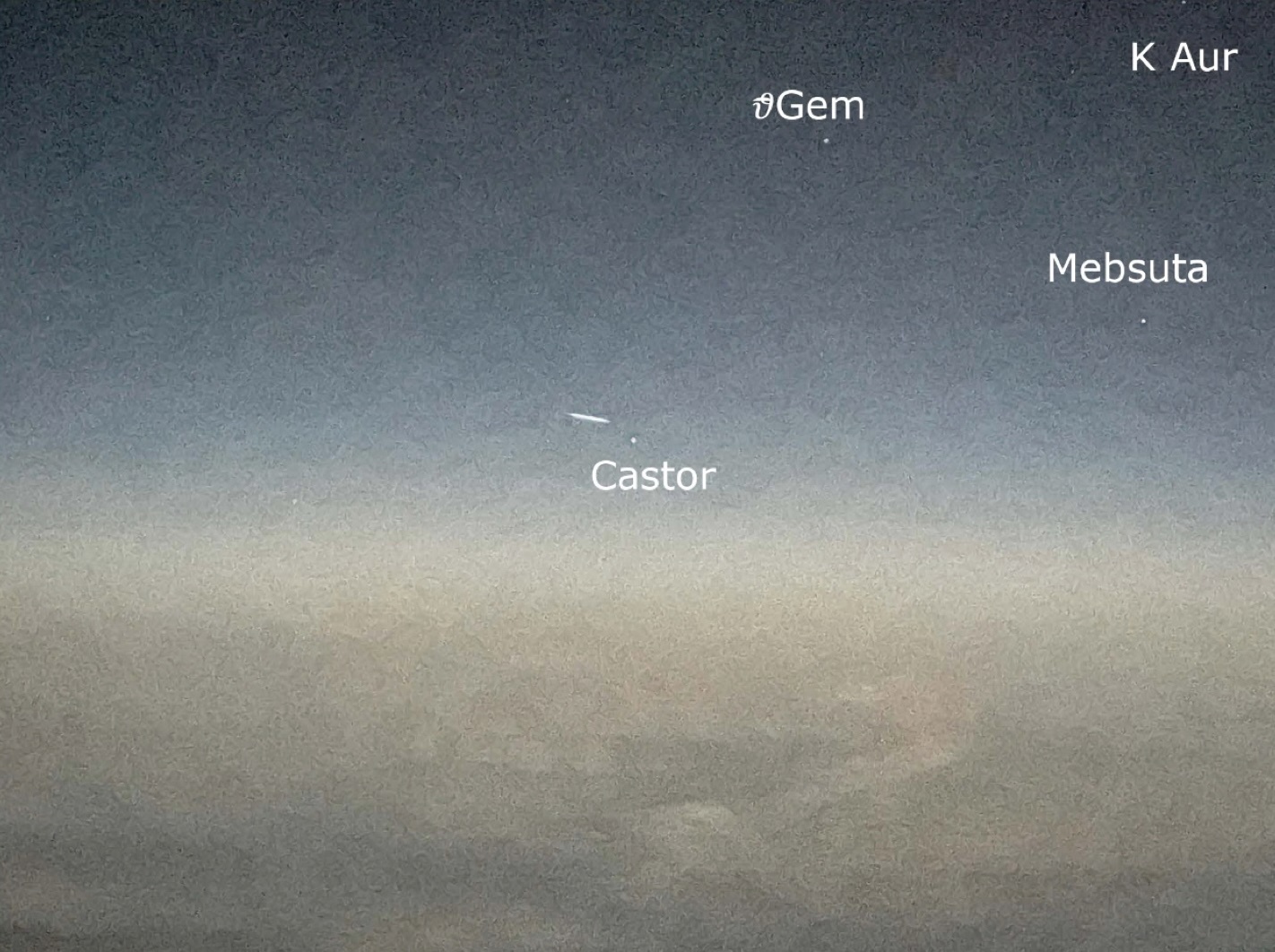
Figure 2. Photo 2 from the iPhone 12 camera taken at 2022-08-10T11:39:24UTC as determined by information embedded in the JPEG metadata. An astrometric solution was unable to be provided by Astrometry.net as it failed to identify the stars in the image due to the camera’s zoom factor distortion. The astrometric solution was provided manually in the second image based on the first image’s solution. At this time, the aircraft was at a latitude of 39.62299 degrees North, and a longitude of 138.404 degrees West.
The cellphone video lasted nearly 16 seconds, but at 12.7 seconds the cellphone was rotated through approximately 90 degrees because of aircraft cockpit window constraints. The recorded intensity of the object then faded for about 0.5 seconds during the cellphone movement and rotation. The image of the object was recovered but the focus was not recovered by the end of the video at 16 seconds. The useful part of the video therefore lasted for the first 12.7 seconds. No stars were recorded in the video because of the short exposure times per frame.
Photometry
The initial sighting was of 4 or 5 very luminous point source objects seen close to the NW horizon with individual objects estimated to have a brightnesses of about 2 or 3x brighter than the International Space Station (ISS) or Venus, with a magnitude of approximately -5. At the estimated distance of 35-75 nautical miles, and assuming isotropic emission, the luminosity of each object was at least 300 kW. There is no photographic evidence for this initial sighting. Analysis of the two photos taken from the leading plane shows independent confirmation of the brightness of the large object, but not the original star-like luminous objects.
The two cellphone JPEG images (from an iPhone 12), shown in Figure 1 and Figure 2, were converted to .fits (Flexible Image Transport System) files for examination using SAOimage DS94 from the Smithsonian Astrophysical Observatory, so that the RGB images could be examined separately. SAOImage DS9 (Mandel 2003) is widely used by astrophysicists for data analysis of astronomical objects against a dark sky background and is an appropriate software package to use in this case. Other image analysis software packages such as ’Forensically’ are commonly used for everyday cellphone photography in daylight (for verification purposes that the image is a ’bona fide’ image and not a ’fake’) but are not as useful in this case, where there is a bright object against a dark sky background, as commonly occurs in observational astronomy. Photometric analysis can be performed with DS9.
To get an approximate value of the brightness of the object, we can examine the photo images and see that the digital pixel values (analog-to-digital units, ADU) are about 250 per pixel within the image of the large object, which is about (115-120) x 13 pixels in size as shown in Figure 1, with a background intensity of 140 per pixel, i.e. the integrated intensity value is about 166,000 ADU.
This compares with an integrated pixel intensity value of 14,000 ADU for the nearby star Castor, which has (Pogson) magnitude (mag) 1.58. Hence, the integrated mag of the large object (11.5 times brighter than Castor) is about 5.5 mags brighter, i.e. a mag of -4.
The large object, as shown in Figure 1, appears to be “cigar shaped”, with scalloped protrusions at either end, with an overall aspect ratio of approximately 116:13. At the time the cellphone images were taken, the distance to the object was not known, but the pilots estimated it to be about 20-30 nautical miles from the plane at roughly the same altitude and within the atmosphere (in this case at a barometric altitude of ~37,000 ft).
The delay between the first sighting from the trailing plane and the first photo from the leading plane is not known but was more than a minute: the captain of the trailing aircraft observed the initial objects in the NW, while the video and photos were taken from the leading plane towards the NNE, as shown by the identification of stars in the background (see discussion of astrometry, above). An approximately 1.5-degree apparent angular size, Figure 3, corresponds to a linear size of about a mile for 30 nautical miles in distance.
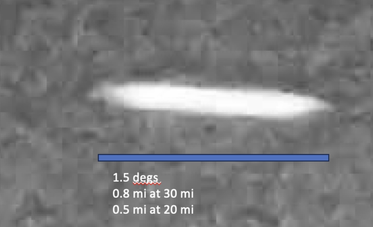
Figure 3. Using the astrometric solution for the background stars, we estimate the apparent angular size of the object as 1.5 degrees in Photo 1. The apparent linear lengths are based on estimated distances of 30 and 20 nautical miles, resulting in linear dimensions of 0.8 and 0.5 miles respectively.
Angular Resolution and Apparent Sizes
The images in Figure 1 and Figure 2 were taken with an Apple iPhone-12. The iPhone- 12 uses lenses of about 2 mm diameter, and therefore has a diffraction limit of about 2 arcminutes (about 2 pixels). No smaller structures can possibly be resolved. The overall size of the cellphone images is approximately 1530 x 2040 pixels, covering 24 x 32 degrees, so that the pixel size (plate scale) is approximately 1 arcminute, smaller than the diffraction limit.
The object appeared in the sky as cigar-shaped, about 116 pixels long (1.5 degrees) and 13 pixels wide in Figure 1, compared with about 5 pixels width for a stellar image. Therefore, the object is only partially resolved in the short (vertical) dimension. In the long dimension, no substructure is visible in the images at the cellphone optical resolution, except for the two ends of the ’cigar’, which both seem to be scalloped on their lower sides (like an aircraft carrier). Alternatively, the object may have apparent extensions which are narrow in height. Photo 1 and the video of the object do, however, show structural subcomponents.
The object was observed at about 2 a.m. local solar time. Assuming that the object was within the atmosphere, at the estimated distance of 20-30 nautical miles away from the aircraft from which the pictures were taken, the luminosity was therefore presumed to be intrinsic to the object. From the perspective of the aircraft the sun was about 30 degrees below the horizon, and the moon had recently set.
In Figure 2, the longitudinal axis of the object ’disk’ was not parallel to the horizon but had an apparent negative pitch angle of about 5 degrees, i.e., leading edge pointing downwards. There was no other indication that the object was descending. Neither is there any indication from the photos or video of any aerodynamic features (e.g. wings, or tail). The downward pitch of about 5 degrees can lead to imaginary features in the low-resolution image, see for example pixel jumps on the topside of the object, but such features are simply caused by 'pixelization' of the image in the cellphone sensor and are not real.
Upon examination of the separated RGB images, SAOImage DS9 shows that there was no change in color across either the narrow dimension or the long dimension – i.e., there was no indication of heat generation anywhere along the length of the object. Some frames of the video do, however, show a gap along the length of the object (see Figure 4 as an example of the observed gap structure).
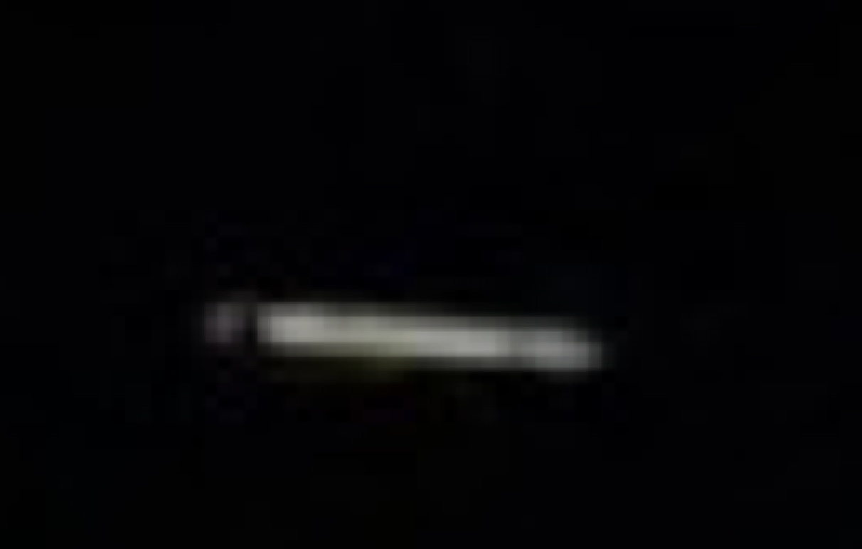
Figure 4. Frame # 26-04 from the pilot video, at about 8 seconds after the first photo, showing a gap structure
The atmospheric (wavelength) dispersion of the image perpendicular to the horizon should amount to several arc seconds between blue and red images, but this is not apparent either in the stellar images or that of the observed object: the cellphone image pixel size is one arc minute, so the atmospheric dispersion is not resolved. Refraction by the atmosphere should, however, be significant, such that stars near the horizon appear to have higher altitude than they would have with no atmosphere (e.g. the actual sun at sunrise or sunset is depressed about half a degree relative to the apparent sun).
Celestial Coordinates and Apparent Velocity
The object was first observed from the trailing aircraft above the North-West horizon, and moved parallel along the horizon towards the North-East, roughly following the flight paths of the two Air Canada aircraft. The object crossed the flight path vector of the leading plane but was by then beyond the view of the trailing plane. The cellphone photos and video were taken from the (leading) flight when the object was above the North-North-East horizon and projected against the constellation of Gemini. There are stars visible in both photo images, though not in the individual video frames because of the short effective exposure times. Astrometry on the stars in the images was performed using ’astrometry.net’ (Dustin Lang et al. 2010).
The following analysis is from the lead aircraft photos and witness report: Astrometry of the stars in Figure 1 shows that the object, as observed from the leading aircraft, was projected on the sky at an apparent position of Right Ascension (RA) 7h 51m, declination (dec) +36d,5 about 2.4 degrees west and 0.5 degrees in elevation south of Jishui, 71-𝜊 Gem. The video shows that the apparent size of the object did not change during the 12.7 second useful interval of the video. Photo 2, however, shows the object angular size to be smaller than in Photo 1, because a ’zoom’ factor has been applied to the second cellphone picture. This zoom factor of about two means that the overall image size of Photo 2 is too wide for application of the astrometric program Astrometry.net, which ’typically’ fails with such wide-angle cellphone images because the program assumes a tangent-plane projection for the images and does not take into account spherical projection effects (Lang 2023), or distortion in the wide-angle cellphone images (i.e. pincushion and/or barrel distortion), visible by inspection of the shape of the horizon.
Manual astrometry of the stars in Figure 2 showed that the object had moved to an apparent position of RA 7h 36m, dec +32d, about 0.5 degrees in elevation above and 1.2 degrees west of Castor. Other stars recorded in Figure 2 are identified as 𝜏-Gem, and κ-Aur. We include an image for the constellation Gemini in Figure 5 for reference. The camera image axes are taken to be roughly altitude-azimuth as shown.
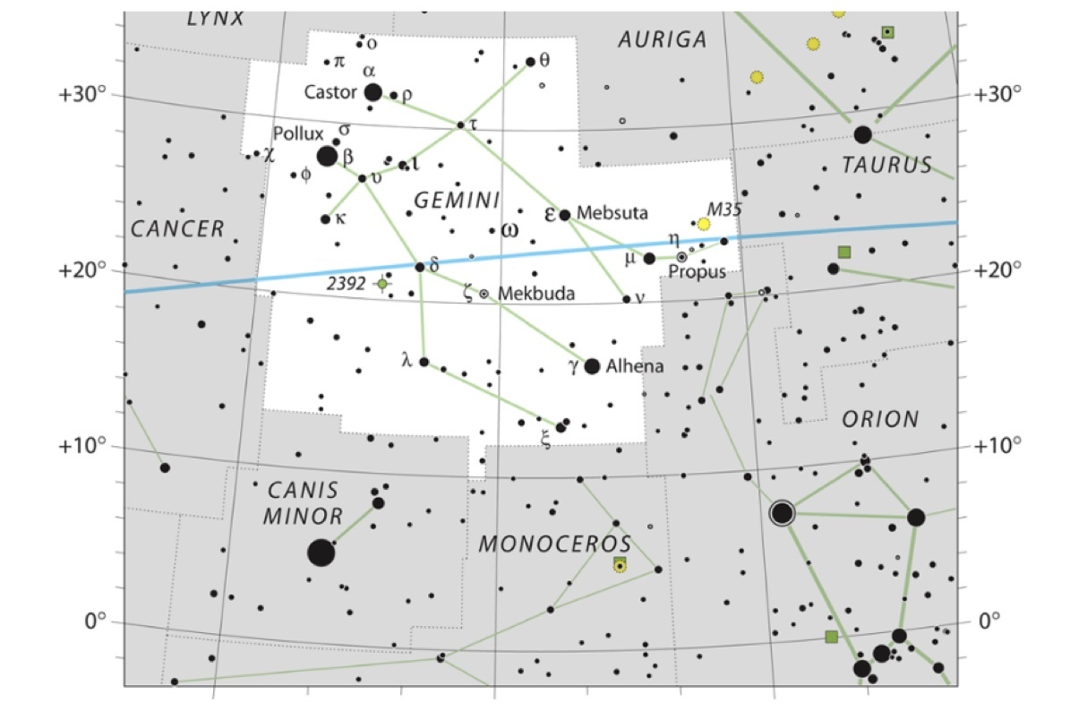
Figure 5. The Gemini constellation (IAU and Sky & Telescope 2015).
The angular distance traversed by the object between the two photos was therefore approximately 4.22 degrees, and the time difference was 16 seconds, as determined from the JPEG files' metadata. Neglecting the motion of the aircraft, the angular rate of motion was thus 0.26 degrees per second, or 90 degrees in just over 2 minutes, in agreement with the witness statement that the object moved 90 degrees across the sky (NW to NNE) in about 2 minutes. The object, as observed from the leading aircraft, had an estimated distance of about 30 nautical miles (somewhat less than the 35-to- 75-nautical mile distance of the initial bright lights seen from the trailing aircraft). At this assumed distance, the angular rate of motion then translated to about 500 mph.
Allowing for the motion of the witness aircraft, the apparent tangential speed of the UAP was thus about 1100 mph, with no measurable radial velocity towards or away from the aircraft.
3. ModelingStarlinkGroup4-26 Orbit Simulation and Visualization
We then investigated whether this sighting could have resulted from a launch of SpaceX/Starlink satellites made earlier the same day (August 10, 2022 at 02:14 UTC) from Pad LC-39A from Kennedy Space Center in Florida USA, i.e. Starlink-54 Group 4-26 (Wall 2022, Sesnic 2022, RocketLaunch.Live 2022). To perform orbital modeling of this satellite group, we use Two-Line Elements (TLEs) for each of the 52 satellites.
Two-Line Elements (TLEs) are a common NORAD format and incorporate the Keplerian elements that describe the orbital variables for the satellites and rocket debris (Kelso 2022, Wikipedia 2023). We first used the Satellite Orbital Analysis Program (SOAP) version 15.4.1 from The Aerospace Corporation (Aerospace), (Aerospace 2020). However, as SOAP is only available to employees of Aerospace and their government customers, we also used a commercially available program, System Tool Kit (STK) version 12.6.0 (AGI/ANSYS 2024) which can perform similar orbit determination analysis as SOAP.6
We also investigated tools capable of providing a visual representation of what the pilots in the aircraft from which the photos were taken would have seen. For this purpose, one of us investigated several tools, settling on the open-source tool Blender 4.0 (Blender 2024) for this purpose due to its price (free), capabilities, and support community even though it is primarily used by the animation community. Blender allowed us to load a CAD model of the aircraft (Goo 2022), model the earth7, and represent the sun's lighting with the ability to perform ray tracing (blender 2023).8
Obtaining TLE, ADS-B and Other Data
TLE's compatible with SOAP were pulled from Celestrak (Kelso 2022) which includes the names of the individual Starlink satellites. Supplemental TLE data for the objects in this Starlink group were also provided by Jonathan McDowell of the Smithsonian Astrophysical Observatory (private communication). Subsequently, Kelso updated CelesTrak's supplemental query of Celestrak’s NORAD archives for “after the fact queries” to extract a Starlink satellite group for a short time frame (7-10 days) using a 7XXXX query format where the XXXX represents the Starlink satellite number (see Figure 6). Hence, a Starlink satellite named 'STARLINK-1234' would be 71234 in Celestrak's supplemental query (Kelso 2022). The combined TLE file used in SOAP is included on our GitHub site (see section 9. Supplementary Materials provided later in this paper). The Starlink satellite name is obtained from Celestrak’s satellite catalog by searching through the catalog for the satellite’s associated with the UTC launch date (Kelso 2024a). A screenshot of the query page containing the inputs for Starlink group 4-26 is provided below in Figure 6. At the time of this article, this is the form
6 While there are several capable orbit simulation tools available, we chose to use STK due to its position in the marketplace and use by aerospace engineering companies.
7 Uses a spherical earth and imagery from NASA (NASA 2004).
8 We elected to forego trying to use the Blender plugin to use the sun for the light source (we do not know the materials used) and elected to simply model the satellites as 3D rectangular shapes with a surface that emits light.
individuals should use with their name and e-mail address to perform a similar query (Kelso 2024b).9,10
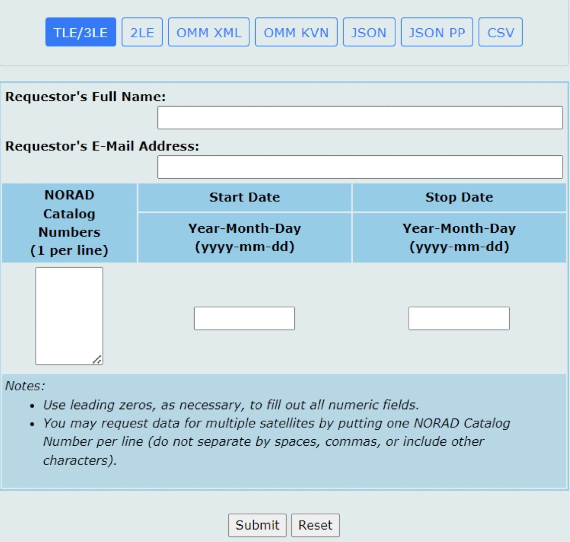
Figure 6. Screengrab of Celestrak’s NORAD archive Supplemental Query Request Form (last accessed in March 2024)
In an a priori pull approach prior to a launch, using for example our Starlink Group 4- 26 launch, the user would use a query formatted as follows:
https://celestrak.org/NORAD/elements/supplemental/sup-gp.php?FILE=starlink-g4- 26&FORMAT=TLE
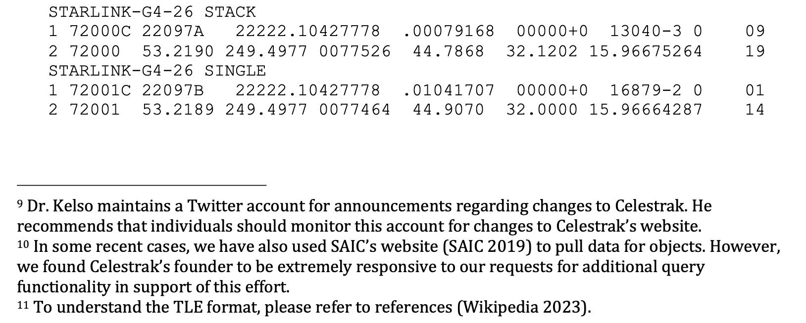
This will return the Starlink payload’s “STACK” and the second stage as the “SINGLE” and use 72000 and 72001 identifiers prior to NORAD ID assignment, appearing as follows:11
After a launch has occurred, one needs to pay attention to the Celestrak satellite catalog to identify the correct NORAD IDs for the objects.
It is important to note the following: "The best we do, by working with SpaceX, is to propagate from the deployment time (when thrusting has stopped) and then fitting that propagation with SGP412 to produce pre-launch ‘SupGP’ data. Within 8-16 hours we usually have individual ephemerides for each satellite that then supplants the pre- launch estimate." (Kelso 2023, Hoots 1988, Vallado, et al. 2012, Kelso 2022). This forces us to manually select the closest UTC time to the photographs for each individual satellite. Recently, Kelso has made further updates to better support providing supplemental data when queries are being made close to but after a launch has been made (Kelso 2024).
To determine the location of the aircraft during their flights, we used the Automatic Dependent Surveillance-Broadcast (ADS-B) data from both flights discussed in the case study. However, for our orbit determination and visualization analysis in SOAP, we were more concerned with aligning our simulation to the flight with photographic evidence (AC356).13 Hence, we only used the ADS-B data from the leading flight, Air Canada (AC536) flight from Kahului, Maui to Vancouver, Canada in our simulations. In addition, since the UTC (Coordinated Universal Time) time for the photographs were available from the photograph's meta-data, we only included the ADS-B for the portion of that flight that was critical for our modeling effort. Hence, the ADS-B data used in SOAP is from 2022-08-10T10:44:22UTC to 2022-08-10T12:49:30UTC.14
The ADS-B data for this flight has barometric pressure-derived altitudes in feet. SOAP, however, requires altitudes above mean sea level (MSL) in kilometers. To accommodate the difference between barometric altitudes and MSL we converted the barometric height values to the Geoid using Orthometric heights from an online conversion tool provided by the National Science Foundation’s Geodetic Facility for the Advancement of Geoscience (GAGE) (EarthScope Consortium 2023).
Finally, the modeling efforts for STK and Blender incorporated a Computer Aided Design (CAD) model of a Boeing aircraft to simulate the appearance of the satellite train more accurately from the aircraft's cockpit. In addition, STK incorporated a CAD model of the SpaceX Falcon 9, while Blender also incorporated a GeoTIFF image of the Earth. The online repository of our modeling results provides these models (see section 9. Supplementary Materials).
Orbit Simulation Results
Using the times that the two photographs were taken we provide the following graphics from SOAP in Figures 7 to Figure 11.
12 SGP is an acronym for Simplified General Perturbations (SGP) where SGP4 is one of the models used by orbit propagation software such as SOAP.
13 ADS-B data for the flights was provided by Dr. Sarah Little.
14 The file “AC536.xlsx” on our GitHub website has the original ADS-B data for the flight and includes all associated numerical calculations used to incorporate AC536 into SOAP’s orbit simulation of Group 4-26.
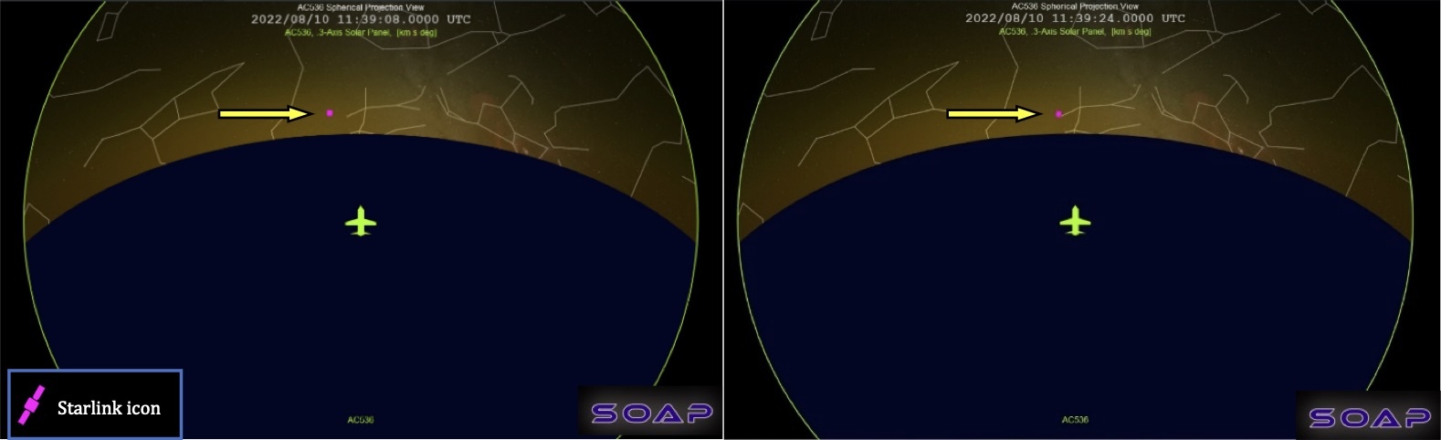
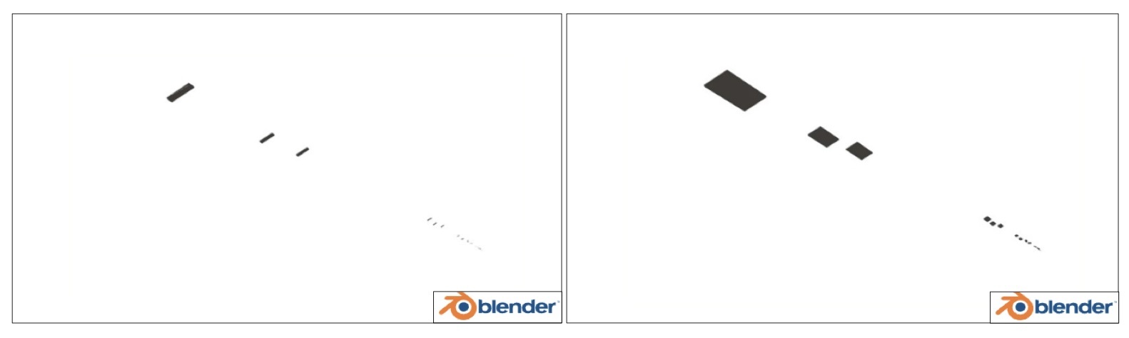
Figures 7a and 7b. Screenshots of SOAP's Spherical Projection View15 viewed looking down on flight AC536 (using SOAP’s yellow aircraft icon with the size exaggerated to make it clearly visible) from above to clearly show the constellations visible to the aircraft above their horizon with respect to the aircraft heading. The satellites (the purple satellite icon) are the positions of all 52 satellites that have been propagated to their orbital location at the same UTC time of the two photographs, yellow arrows are included to help identify their location in the screenshots. Fig 7a, the image on the left has the satellites propagated to the UTC time for the first photograph (Aug 10th, 2022 11:39:08UTC), while Fig 7b, the image on the right has the satellites propagated to the time for the second photograph (Aug 10th, 2022 11:39:24UTC). The satellites are clearly near Gemini.
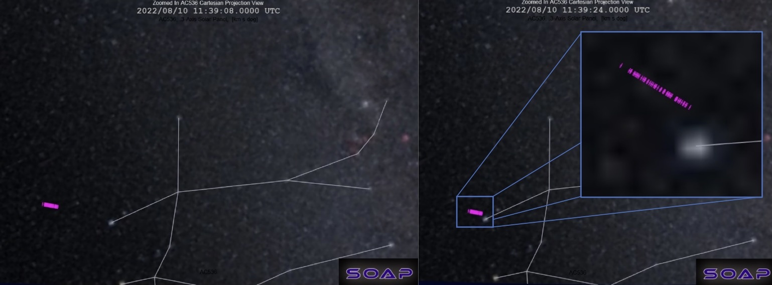
Figures 8a and 8b. Screenshots of SOAP’s Cartesian Projection View of the zoomed in relative locations of the satellites (same purple satellite icon as used in Figures 7) as viewed from the cockpit of AC536 aircraft at the time of the photographs, again clearly showing its location with respect to Gemini. Fig 8a is from the UTC time for the first photograph (Aug 10th, 2022 11:39:08UTC), while Fig 8b has the satellites propagated to the time for the second photograph (Aug 10th, 2022 11:39:24UTC). We also include in 8b a further zoomed in insert to show the gaps in between the satellites as viewed from flight AC536’s cockpit.
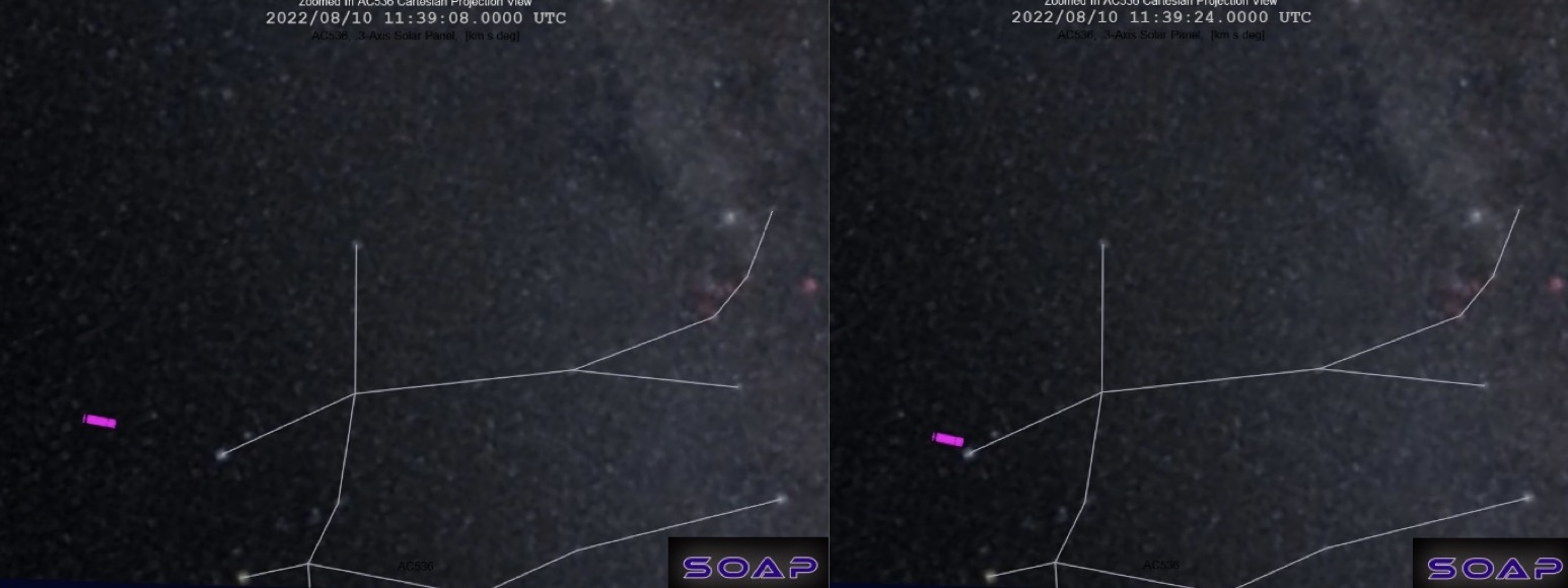
Figures 9a and 9b. This figure is a repeat of Figures 8a and 8b SOAP’s Cartesian Projection View of the zoomed in relative locations of the satellites (same purple satellite icons). However, this time the aircraft’s position has an additional 0.8 km included in the altitude to account for potential barometric altitude error. The zoomed in insert in Figures 8b has not been included in Fig 9b. These screenshots are provided to demonstrate the imperceptible visual effect of an altitude error in our results.
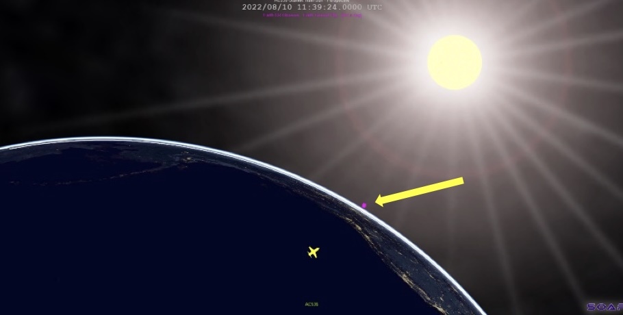
Figure 10. Screenshot from SOAP’S spherical view with the Starlink satellite train propagated to the time of the second photograph showing it in full view of the sun. The yellow arrow is included to aid finding the location of the satellites in this image. The yellow aircraft icon for AC536 shows the direction the aircraft was traveling and that it is still in the Earth’s shadow, where the white line along the Earth’s limb is the day/night terminator.
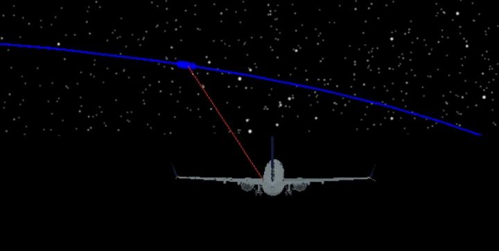
Figure 11. Screenshot from STK showing the Starlink satellite train (blue satellite icons) propagated to Aug 10th, 2022, 11:39:08UTC, the time of the first photograph from the perspective of the AC536 aircraft (depicted using a CAD model (Goo 2022)). The path of the satellite train is also blue.
Finally, as the ADS-B barometric altitude values could be off by as much as 2500 feet at altitude (S. Narayanan 2022), we provided Figures 9 to show no significant difference in the simulated satellite train's apparent location with an additional 2500 feet added to the MSL altitude (+0.8 km). Further, looking at the processed values from the Python script output files one notices that the potential for an altitude error leads to negligible relative position differences to the satellites based on how far they are from the aircraft. The screenshots at the time of photo 2 show that the train is almost on top of 𝛼-Gem (Castor). Additional screenshots showing the locations when an additional altitude error is added to the aircraft demonstrate negligible change in the relative location of the satellite train for both photos.
Blender Visualization Results
Blender 4.0.1 was used to attempt to create a realistic cockpit view of the Starlink train using ray tracing (Blender 2023). To place the Starlink train in the correct location as viewed from the cockpit, we translated our look angle coordinates into cartesian coordinates centered on the CAD model of a Boeing aircraft. Size estimates of a Starlink satellite were obtained from two different references (reddit users 2023) and (Forrest 2020), neither of which are official SpaceX/Starlink publications. This is an issue but is the best current information that we must work from.16
Figures 12 shows a zoomed in of Starlink satellites with the solar arrays in the stowed and deployed (open-book) configuration, respectively. These images also document the relative locations, rotation angles (X-axis is -170 degrees, Y-axis is 31.92 degrees, and Z-axis is -10 degrees), and sizes for the model used in this paper.17
Figures 12a and b. Screengrabs of our simple Blender model of Starlinks using Blender’s “Cube” for simplicity. In Fig 12a, represents the satellites with their solar arrays in the stowed for launch configuration, the Cubes are dimensioned to 2.8 meters in width by 1.4 meters in length and 0.2 m in height (or thickness) representing the satellites in the stowed solar array configuration. In Fig 12b, the open-book configuration, the Cube representing each satellite, has had the length dimension modified by adding an additional 10 meters to change the length to 11.4 meters to represent their solar arrays being deployed (the “open-book” configuration) while they are in their orbit boost phase. In both images, Blender camera’s viewpoint has been moved from within the aircraft’s CAD model to a mere 161.2 meters from the nearest satellite (Starlink-4479) to show the change in observed surface area in this orientation. The orientation was selected to have the solar array extend into the direction of travel of the satellite train, and the Y-rotation angle is the same angle as the average of the sun’s grazing angle for each Satellite as determined by our Python script. Each satellite has been placed at the correct relative distance from the AC536 aircraft as were calculated by our Python script from the first photo’s UTC time. The subsequent satellites in view are Starlink-#s 4304, 4484, 4476, 4480, 4545, and so forth. From this closer viewpoint, the clustering of satellites as the cause for the observed gaps is easily observed.
Figure 13 displays the relative location of the satellite train from within the cockpit, not considering local roll-pitch-yaw aircraft dynamics as there was no data to suggest significant perturbations to the ADS-B data for these axes.
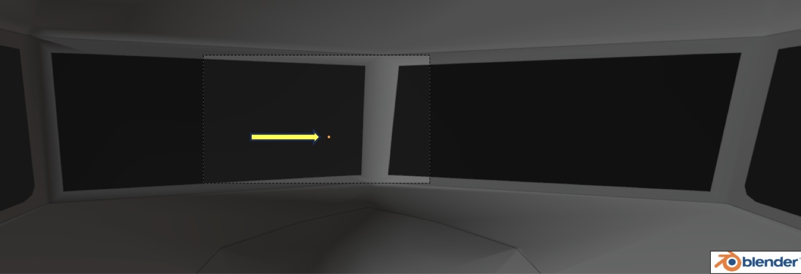
Figure 13. Screengrab showing the location of the Starlink train (the yellow dot just to the right of the yellow arrow) as viewed from the cockpit at the time of photo 1 as determined from ADS- B and Group 4-26 TLE data and transformed into cockpit view coordinates. The grey box surrounding this area of the screen is the location of Blender’s camera view, and represents the area that is rendered, as shown below in Figure 14 and Figure 15.
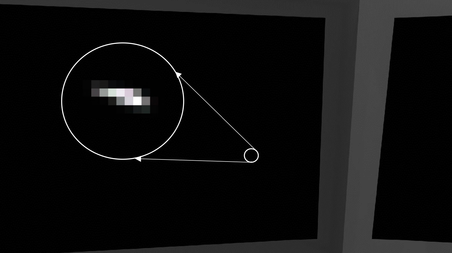
Figure 14. Rendering of the Starlink train in the open-book solar array configuration from one of our rendering experiments. The insert shows a zoomed in view of the rendering with these settings. The rendered result only shows two satellites with the remainder hidden behind these two.18 It took 9 minutes and 50.48 seconds to render this image on the HP Omen laptop that was used for these experiments.19
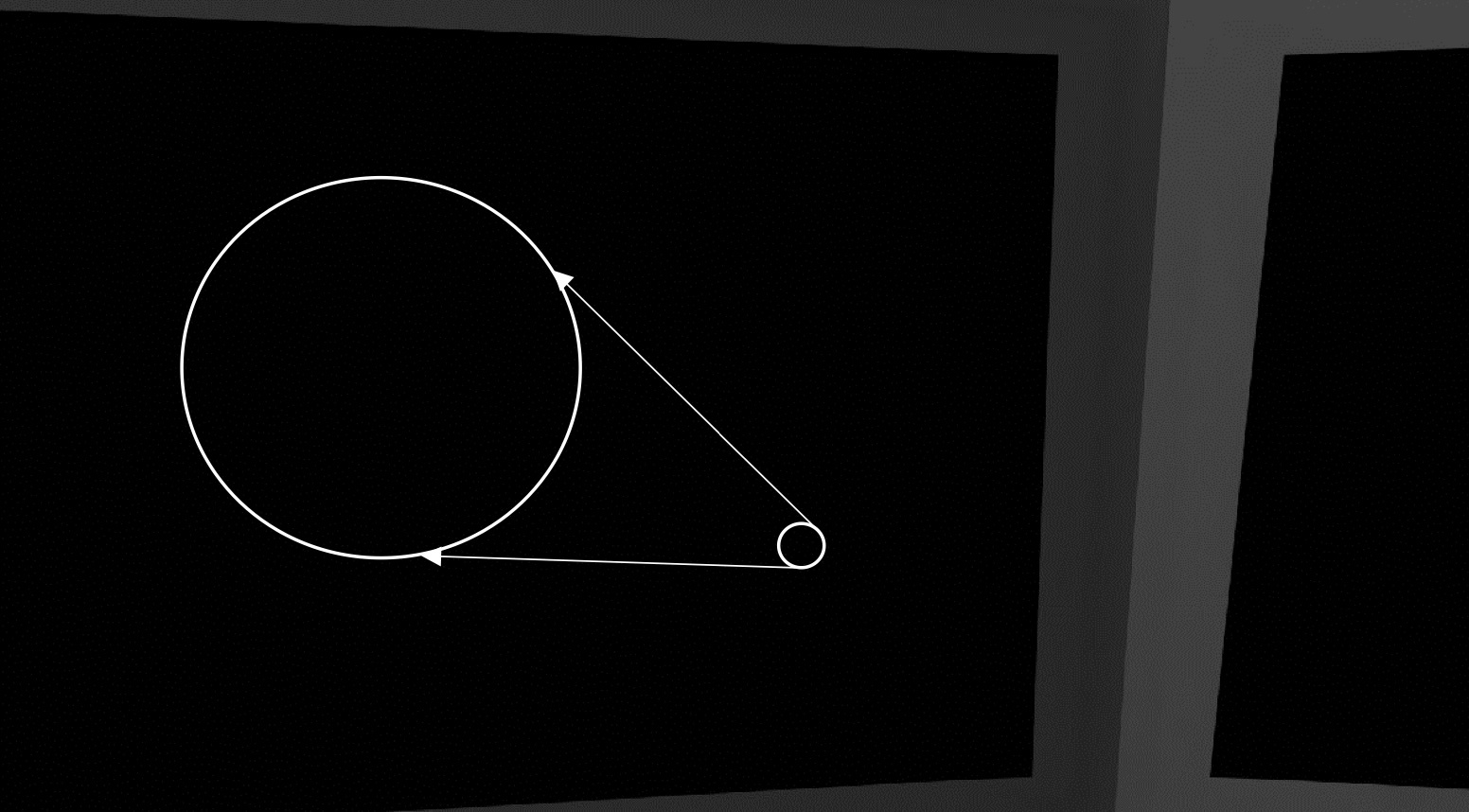
Figure 15. Rendering of the Starlink train in the stowed, undeployed solar array configuration from one of our rendering experiments. The insert shows a zoomed in view of the rendering with the same rendering settings as used in the open-book configuration. Here we see for this experiment that nothing is observed.20 There are, however, experiments where a very faint object is visible. Due to the time to render each of these images on our hardware, and after rendering several different experiments with variations in Starlink orientation, emission intensity, noise levels, number of samples and others, we felt that we had in principle demonstrated the type of analysis that should be performed. We further concluded that this work should be revisited in the future using specialized space-based rendering software such as that from the OpenSpace Project (OpenSpace Team 2023).
Figure 14 and Figure 15 are ray-traced renderings of the open-book and stowed (undeployed) Starlink train at the distances observed at the time of photo 1. To do the renderings, Starlinks are configured as emission surfaces, and in both cases had the strength set to a million with 8192 samples.
These experiments, while not definitive, suggest that the solar arrays had to have been deployed for the satellites to have been observed by the pilots in both aircraft.
Geometry of the Satellite Train's Observation
Extracting Earth Centered Inertial (ECI) based state vectors for the aircraft, the satellites, and the sun at the time of the photographs from SOAP is straightforward.21
18 Details for the rendering settings for this experiment can be found on our GitHub site in the file STLNew_ph1-rotated-open.blend
19 We used a 3.2 GHz AMD Ryzen 7 5800H with Radeon Graphics, and an NVIDIA GeForce RTX 3060 GPU at driver version 546.26 with 7.34 GB of Video RAM.
20 Details for the rendering settings for this experiment can be found on our GitHub site in the file STLNew_ph1-rotated-closed.blend
21 This is a “copy to clipboard” option available within SOAP when displaying each platform’s (sun, aircraft, or satellite) data view, which were each saved to a different ascii text file.
We want to do this to compare our geometry to the case study. Figure 16 shows the vector geometry of a Starlink satellite train relative to an aircraft.
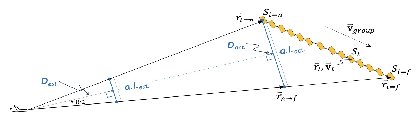
Figure 16. This is a vector diagram representation of the location of the 𝒊𝒕𝒉 Starlink satellite in the train with 𝒊 = 𝒏 for the nearest visible satellite in the train, and 𝒊 = 𝒇 for the furthest visible satellite in the train, as viewed from the cockpit. The diagram is drawn in relation to the common method for calculating the size of a rigid object at an estimated distance Dest. and is represented by the solid blue arrow ending at the estimated apparent length a.l.est. which is also in blue font. Dest. is perpendicular to a.l.est.. The apparent actual distance, Dact. is represented by the continued dashed blue arrow that starts at the aircraft and ends at the actual apparent length a.l.act. which is also in blue font. Dact. is perpendicular to a.l.act.. Hence, the actual apparent length starts at the distance from the aircraft to the nearest satellite with state vector 𝐫⃑𝒊$𝒏, 𝐯)⃑𝒊$𝒏 relative to the aircraft and is represented as 𝑺𝒊$𝒏 in the diagram. The actual apparent length terminates along the line of sight (LOS) to the last visible satellite in the group with the position vector is 𝐫⃑𝒊$𝒇, so that the actual apparent length is perpendicular to the actual apparent distance and is the projection of the nearest visible satellite's position vector onto the furthest visible satellite’s position vector 𝐫⃑𝒏→𝒇. The apparent velocity of the group (𝐯)⃑𝒈𝒓𝒐𝒖𝒑) would be moving from the upper left to the lower
right in the field of view. The 𝒊𝒕𝒉 Starlink satellite is 𝑺𝒊 with state vector 𝐫⃑𝒊, 𝐯)⃑𝒊. The nearest satellite is represented as 𝑺𝒊$𝒏, and 𝑺𝒊$𝒇 depicts the furthest satellite. Likewise, the nearest Starlink's position is 𝐫⃑𝒊$𝒏, and the furthest satellite's position vector is 𝐫⃑𝒊$𝒇. The angle θ between these LOS position vectors is the actual apparent length in degrees.
The object's estimated apparent length in degrees (the angle θ) was estimated from the photo to be about 1.5 degrees, with a pilot-estimated distance Dest. of ~20 to 30 miles. The apparent length a.l.est. at these distances was estimated to be about a mile at 30 miles in distance (1.61 km) in the case study's photometry section. The actual apparent length is identified in the diagram as a.l.act., where the value for the actual apparent length in degrees is calculated from,
𝑟⃗ ∙ 𝑟⃗ cos𝜃=! "⇒
|𝑟 |/𝑟 / !"
𝑟⃗∙𝑟⃗ 180% 𝜃 = cos#$ 1 ! " 2
|𝑟 |/𝑟 / 𝜋 !"
Note that for the aircraft, we have a 'Smooth Route' option selected, where SOAP employs an algorithm that “banks the aircraft” between route points, rather than performing abrupt changes in direction.22 Aircraft relative state vectors for each satellite are computed as,
22 It is possible this option can introduce variations in the relative position of the satellites as viewed from the cockpit with ADS-B data that is not updated say on the order of every minute. Hence, we did experiments with this option disabled as well. It does add measurable changes to the state vector of the aircraft.
𝑟⃗ = 𝑟⃗ − 𝑟⃗
& ()* +% ,-. & &! /0/1 ,-.&! /0/1
𝑣⃗& ()* +% ,-. = 𝑣⃗& &! /0/1 − 𝑣⃗,-.&! /0/1
Recalling that the magnitude of a vector is given by,
|𝑟| = 9𝑟 3 + 𝑟 3 + 𝑟 3 245
From these extracted state vectors, in addition to calculating the apparent lengths (a.l.act. and a.l.est.) using Earth-Centered-Earth-Fixed (ECEF) coordinates, we wished to convert the coordinates to be relative to the aircraft. We used various coordinate systems for the aircraft, such as NTW (Nadir-Track-Wing) coordinates, settling on cockpit relative representation below. NTW was used for calculating the sun grazing angle N-axis lies in the orbital plane pointed at the Earth, T is tangential to the orbit along the velocity vector, and W is normal to these axes.23
Hence, based on the geometry in Figure 16 above, and Figure 17 below, we derive the sun’s grazing angle and the apparent length of the satellite train. To do this we transform ECEF coordinates for the aircraft and the sun to be relative to each of the Starlink satellites in NTW. We then calculate the angle between each of these vectors, using the same vector dot product equation for (θ) above. The grazing angle (φ) in degrees is then given by,
φ = (180 - θ)/2.
Figure 17 uses the same diagram format found in (Fankhauser, Tyson and Askari 2023) to show the grazing angle with the angles between the sun and the aircraft relative to the satellite.
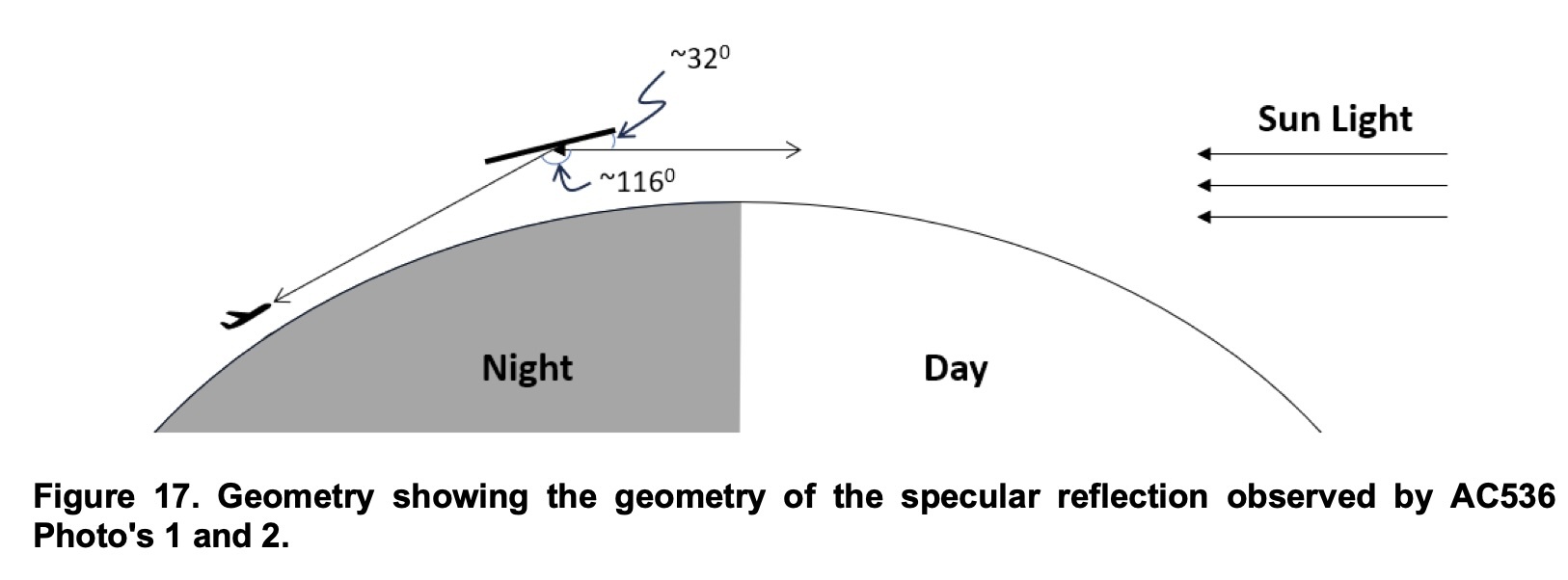
Figure 17. Geometry showing the geometry of the specular reflection observed by AC536 Photo's 1 and 2.
To simulate the location of the Starlink train in the cockpit, we also needed to transform ECEF from SOAP into aircraft heading relative ENU (East-North-Up) coordinates. We define the “look angle” as positive from the heading clockwise and negative counterclockwise from the aircraft’s heading. The elevation angle is defined to be positive in the “up” direction and negative in the “down” direction. Absent information regarding the real-time roll-pitch-yaw status of the aircraft we assume these perturbations are non-existent in the following derivation of the transformations from ECEF to ENU with a heading angle rotation correction.
23 Note that we tested using both NTW and RSW coordinates where RSW is like the roll-pitch-yaw coordinate system (RPY), where R→yaw, S→roll, and W→pitch. As there was no difference in the grazing angle results, we elected to keep just the NTW calculations in our script. For a description of the difference between these satellite coordinate systems, we refer the reader to (Vallado 2013) pgs. 155- 158.
To transform ECEF into local ENU coordinate system at the aircraft's location we use
the aircraft's latitude (φ), and longitude (λ). The altitude of the aircraft is embedded in
the ECEF coordinates extracted from SOAP. The transformation from ECEF to ENU
coordinates involves rotating first about the Z-axis by (−λ) to align the prime meridian
with the local meridian, then about the transverse axis by (6 − 𝜙) to align the up 3
direction with local vertical. The resulting rotation matrix to ENU is,
−sin𝜆 −sin𝜙cos𝜆 cos𝜙cos𝜆 𝑅/0/1→/89 = 𝑅:𝑅; = = cos𝜆 −sin𝜙sin𝜆 cos𝜙sin𝜆A.
0 cos𝜙 sin𝜙
Each of the columns of this rotation matrix define the three-unit vectors 𝑒D, 𝑛D, and 𝑢I respectively. Following the ECEF to ENU conversion we then need to account for the aircraft’s heading to provide a cockpit view. We rotate the East and North axes by the negative heading angle to account for our desire to have the look angle be positive in the clockwise direction and negative in the counterclockwise direction.
cosK−𝜃<),=&!> L sinK−𝜃<),=&!> L 0
𝑅<),=&!> = J−sinK−𝜃<),=&!>L cosK−𝜃<),=&!>L 0M ⇒ 001
cosK𝜃<),=&!> L − sinK𝜃<),=&!> L 0 J sinK𝜃<),=&!> L cosK𝜃<),=&!> L 0M
001
Finally, the look angle (𝛼*%%?) and the elevation angles (𝑒𝑙) in degrees are calculated
from the following equations,
𝛼*%%? = 𝐴𝑟𝑐𝑇𝑎𝑛2K𝐸/0/1→/89→<),=&!>,𝑁/0/1→/89→<),=&!>L180 𝜋
𝑒𝑙= 𝐴𝑟𝑐𝑇𝑎𝑛2K𝑈/0/1→/89→<),=&!>,𝐷<%(&5%!+,*L180 𝜋
with 𝐷<%(&5%!+,* given by,
𝐷<%(&5%!+,* = 9𝐸/0/1→/89→<),=&!>3 + 𝑁/0/1→/89→<),=&!>3
To obtain these results we wrote three different Python scripts (with the support from OpenAI's ChatGPT), the first of which translates the SOAP Starlink ephemerides that were copied into ASCII files, into comma-delimited (csv) files. The second script then processes each of the csv files to methodically calculate for each satellite and aircraft file the sun grazing angle, the apparent length, and the heading corrected locations. A third python script contains the rotations from (Vallado 2013). Table 1
provides a summary of our results from processing the SOAP extracted data from both photos.
Table 1. Summary of results from processing SOAP simulation extracted data with the route smoothing algorithm off. The output-analysis.xlsx excel spreadsheet provided on our GitHub site (see section 9 later in this paper) also includes data from when this SOAP algorithm was enabled.
Quelle: University of Utah
Fortsetzung: 2